Walkthrough on the edge of stochastic stability of neural networks.

Dynamics of SGD at the edge of Lyapunov stability.

1 · Classical SGD update.

\[ \theta_{t+1}=\theta_t-h\,\nabla L_{B_t}(\theta_t) \]

At every iteration, SGD updates the iterate with an unbiased estimate of the gradient. The type of SGD is only the batch-sampling rule: online SGD uses one example; minibatch SGD uses \(B\) examples, drawn with or without replacement. For simplicity, let's just consider the sample batches are drawn i.i.d.

2 · Does current literature about stability of SGD predict what happen in neural networks?

The dynamics of SGD are classical under Lipschitz assumptions, yet that theory does not predict what we see in deep networks. This tutorial recaps the quadratic picture, lists the observations it cannot explain, and then turns to scalar and high-dimensional models that do match the practical behaviour.

3 · SGD on a quadratic loss.

Start with one coordinate and a quadratic loss whose curvature \(a_t\) is redrawn i.i.d. each step:

\[ L_t(x)=\tfrac12\,a_t\,x^2,\qquad a_t\sim\mathrm{i.i.d.} \]

Writing the SGD update step with additive Gaussian noise:

\[ x_{t+1}=x_t-h\nabla L_t(x_t)+\sigma\xi_t=(1-h a_t)\,x_t+\sigma\xi_t \;=\; A_t\,x_t+\sigma\xi_t \]

If the curvature is a fixed number \(a\), this is ordinary gradient descent: the iterate is a geometric sequence, so it converges when \(h<2/a\) and diverges when \(h>2/a\). There is only one threshold.

For SGD the sampled curvature \(a_t\) and multiplier \(A_t\) are random. The stationary distribution of \(x\) is then a property of the step size \(h\) and the distribution of \(A\). Convergence or divergence is a statement about moments of that distribution:

Mean-square stability. \(\mathbb{E}[A^2]<1\). The second moment of \(x\) decays, so the variance stays finite.
Lyapunov stability. \(\Lambda=\mathbb{E}\log|A|<0\). A typical trajectory still goes to zero. This is weaker: almost every path returns to the origin even when some moments do not.

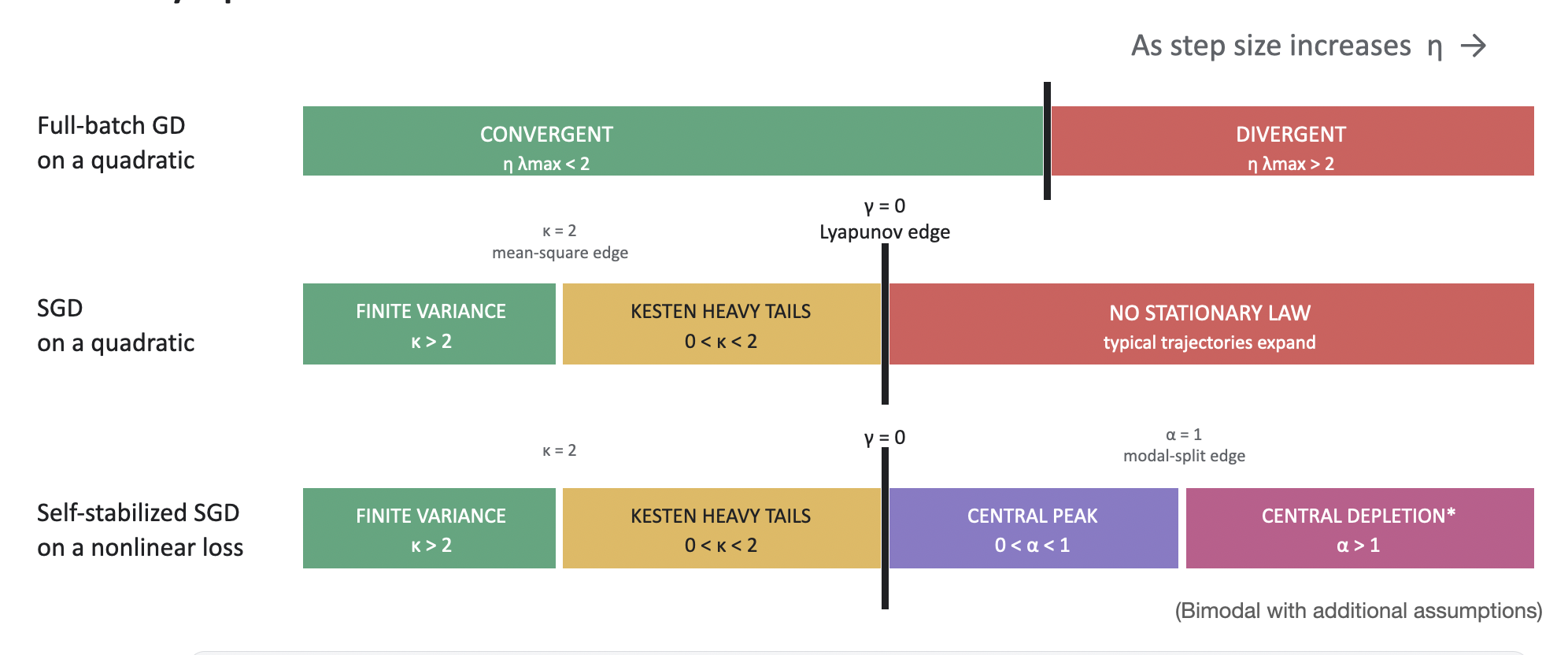
Between the two edges the iterate is heavy-tailed: almost every path returns to zero, while the variance blows up.

Kesten's theorem names the tail of this random walk. If the curvatures are i.i.d.\ and the Lyapunov exponent is negative,

\[ x_{t}=(1-h a_{t})\,x_{t-1}+\sigma\xi_{t},\qquad a_{t}\sim\nu,\quad \xi_{t}\sim\mathcal{N}(0,1),\qquad \Lambda=\mathbb{E}\log|1-h a|<0 \]

then a unique stationary distribution exists, and it has a power tail whose index \(\alpha>0\) is the unique positive root of

\[ \mathbb{E}\big[|1-h a|^{\alpha}\big]=1 \]

\[ \mathbb{P}(|x_{\infty}|>x)\;\sim\; C(\sigma)\,x^{-\alpha}\qquad\text{as }x\to\infty \]

The power matches the tail index of the stationary distribution. A positive root exists only while \(\Lambda<0\). So \(\alpha\) slides from large (nearly Gaussian) through \(\alpha=2\) at the mean-square edge down to \(\alpha=0\) at the Lyapunov edge, where the stationary distribution is gone.

SGD on a quadratic across increasing curvature: trajectories, histograms and tail index — Left to right, growing step size \(h\). Top: iterates inside the quadratic. Middle: the histogram of \(x\). Bottom: the tail index \(\alpha\). The two vertical lines are the mean-square edge (\(\alpha=2\)) and the Lyapunov edge (\(\alpha=0\)). Past the second line there is nothing left to converge to.

This seems quite convincing and seems to give a full picture.

4 · The gap in prediction using exact quadratics

Training an MLP on CIFAR-10 with SGD at the edge of stochastic stability, we freeze a late checkpoint \(\theta_\star\), take the top Hessian eigenvector \(u_1\), and continue from there. The loss has already collapsed. In a late tracking window the occupancy of \(\langle\theta-\theta_\star,u_1\rangle\) is still two lobes with a gap at the checkpoint.

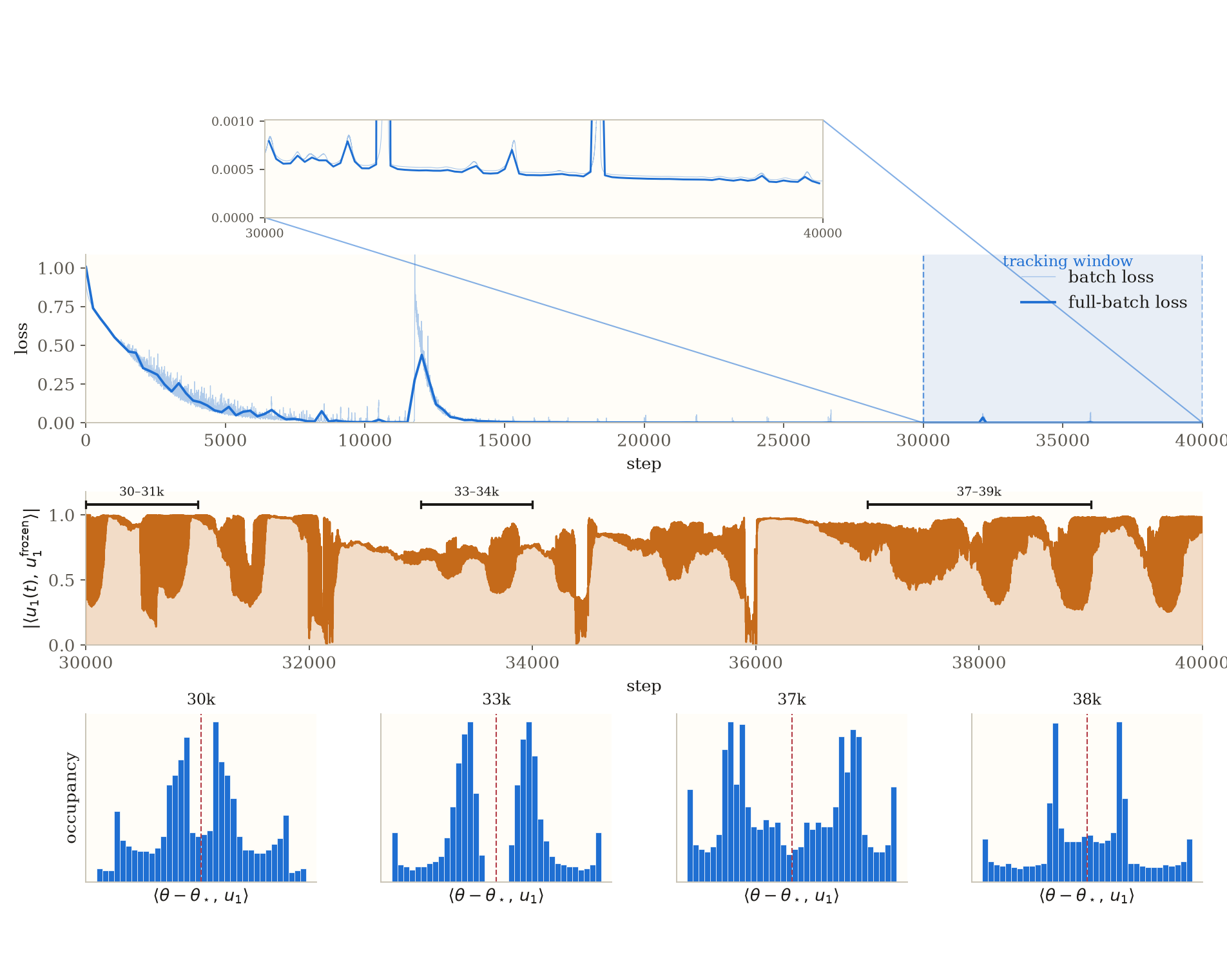
CIFAR-10 MLP: late-training loss, u1 alignment, and two-lobe occupancy along u1 — The distribution is bounded, and it has split into two lobes with a gap at the checkpoint. Top: full-batch loss with a late tracking window. Middle: alignment of \(u_1(t)\) to the frozen top direction. Bottom: occupancy of \(\langle\theta-\theta_\star,u_1\rangle\) in two-well chunks.

Measuring the Lyapunov exponent along that direction we get,

\[ \Lambda=\mathbb{E}\Big[\log\big|1-\eta\,u_1^{\top}H\,u_1\big|\Big]=+0.023 \]

This violates the first assumption of Kesten's random walk theorem which requires negative Lyapunov exponent. \(\Lambda>0\) means \(\mathbb{E}[|A|^\alpha]=1\) has no positive root. Kesten says: no stationary distribution, the iterate leaves. Instead it is bounded, and it is bimodal.

So the linear part really is expanding, and something outside the linear part is holding the iterate in. As you can already guess, the exact quadratic picture is flawed here: the natural next step is to ask whether a higher-order polynomial approximation of the loss can predict these dynamics.

We now turn to three labs that build that missing piece — first as a scalar nonlinearity, then as a matrix effect, then back on the network.

5 · The harmonic instability edge.

Keeping the same scalar update. Only the loss changes: replace the quadratic by a quartic, so the step picks up restoring terms.

\[ x_{t+1}=(1-h a_t)\,x_t+\alpha x_t^3-\beta x_t^5+\sigma\xi_t \]

Near zero this is still the Kesten map \(A_tx_t+\sigma\xi_t\). Once the iterate is pushed out, the higher terms pull it back, so an expanding linear multiplier no longer means escape. Raise \(h\) past the Lyapunov edge and the same path that used to diverge settles into two lobes.

The linear map has one more threshold after Lyapunov. Mean-square is \(\mathbb{E}[A^2]<1\). Lyapunov is \(\mathbb{E}\log|A|<0\). Harmonic stability is the inverse moment of the same multiplier:

\[ H(h)=\mathbb{E}\big[\,|1-h a|^{-1}\,\big] \]

The origin is harmonically unstable once \(H(h)<1\). The harmonic stability limit \(h_H\) is the first step size at that crossing, \(H(h_H)=1\). Past Lyapunov a typical path already expands near zero; past \(h_H\) the return becomes rare, so the restoring terms hold the iterate in two wells instead of a spike at the origin. (If the distribution of \(a\) can hit \(1/h\), the expectation diverges and one reads \(h_H\) from the histogram: the first \(h\) at which the cloud is bimodal.)

The histogram of the cloud then goes from a spike at \(0\), through a tent after Lyapunov, to two wells past \(h_H\). That is the strip below: only the step size changes.

Drag the step size across the edges, then turn the nonlinear terms on and off. Open this lab alone.

In this work, we first define a new edge to characterize this stability threshold, which we call the harmonic instability edge.

Left to right, growing step size \(h\). Spike at \(0\), then a tent after Lyapunov, then two wells past the harmonic instability edge \(h_H\). Only \(h\) changes.

6 · High-dimensional linear regression.

We extend the toy setup to 2-dimensional linear regression where the batch samples are drawn i.i.d from a Gaussian distribution. Each step picks a minibatch \(\mathcal B_t\) of size \(B\) and forms the batch Hessian from those covariates. We add an isotropic self-stabilization coefficient to observe the iterate dynamics in the post-Lyapunov regime. Note that since the Gaussian covariates are drawn i.i.d, the linear matrix product are non-commutative and hence a non-trivial extension of the scalar case above.

\[ x_{t+1}=(I-h H_t)\,x_t-h\Big(\tfrac{c_{4,t}}{6}\|x_t\|^2+\tfrac{c_{6,t}}{120}\|x_t\|^4\Big)x_t+\sigma\xi_t,\qquad H_t=\frac1B\sum_{i\in\mathcal B_t}z_i z_i^\top,\quad z_i\sim\mathcal N(0,\Sigma),\quad \Sigma=\mathrm{diag}(\mu_1,\mu_2) \]

In the diagram below, we plot iterate histogram distribution of the cooridnates x1 and x2.

Pick a batch preset, hit Run, compare the two stability readouts. Open this lab alone.

7 · Back to the network.

Now let’s see the dynamics of SGD. We train several neural networks to completion. Then, using a different batch size and step size, we run SGD iterations from those trained checkpoints and plot the iterate histogram in the top two Hessian eigenvector directions.

Choose a checkpoint pack, sweep step size or batch, then run. Open this lab alone.

8 · Conclusion.

Full-batch GD on a quadratic has a single threshold where it converges or it diverges. SGD on the same quadratic has a tail spectrum that depends on the step-size and batch distribution. Self-stabilized SGD on a nonlinear loss does something new. After the Lyapunov edge the iterate stays bounded, and a new spectrum appears, organized by the negative-moment root \(\alpha\): a central peak while \(0<\alpha<1\), then central depletion once that root crosses \(\alpha=1\). That last crossing is the modal-split edge — the origin empties and, under the usual extra assumptions, the cloud becomes two lobes.

Spectrum of SGD: full-batch GD, quadratic SGD, and self-stabilized SGD as step size increases — As the step size grows. Self-stabilized SGD continues past Lyapunov: a central peak, then central depletion at the negative-moment root \(\alpha=1\).